A 12-step visual guide to understanding NeRF (Representing Scenes as Neural Radiance Fields)
NeRF overview — Image by AuthorA Beginner’s 12-Step Visual Guide to Understanding NeRF: Neural Radiance Fields for Scene Representation and View SynthesisA basic understanding of NeRF’s workings through visual representationsWho should read this article?This article aims to provide a basic beginner level understanding of NeRF’s workings through visual representations. While various blogs offer detailed explanations of NeRF, these are often geared toward readers with a strong technical background in volume rendering and 3D graphics. In contrast, this article seeks to explain NeRF with minimal prerequisite knowledge, with an optional technical snippet at the end for curious readers. For those interested in the mathematical details behind NeRF, a list of further readings is provided at the end.What is NeRF and How Does It Work?NeRF, short for Neural Radiance Fields, is a 2020 paper introducing a novel method for rendering 2D images from 3D scenes. Traditional approaches rely on physics-based, computationally intensive techniques such as ray casting and ray tracing. These involve tracing a ray of light from each pixel of the 2D image back to the scene particles to estimate the pixel color. While these methods offer high accuracy (e.g., images captured by phone cameras closely approximate what the human eye perceives from the same angle), they are often slow and require significant computational resources, such as GPUs, for parallel processing. As a result, implementing these methods on edge devices with limited computing capabilities is nearly impossible.NeRF addresses this issue by functioning as a scene compression method. It uses an overfitted multi-layer perceptron (MLP) to encode scene information, which can then be queried from any viewing direction to generate a 2D-rendered image. When properly trained, NeRF significantly reduces storage requirements; for example, a simple 3D scene can typically be compressed into about 5MB of data.At its core, NeRF answers the following question using an MLP:What will I see if I view the scene from this direction?This question is answered by providing the viewing direction (in terms of two angles (θ, φ), or a unit vector) to the MLP as input, and MLP provides RGB (directional emitted color) and volume density, which is then processed through volumetric rendering to produce the final RGB value that the pixel sees. To create an image of a certain resolution (say HxW), the MLP is queried HxW times for each pixel’s viewing direction, and the image is created. Since the release of the first NeRF paper, numerous updates have been made to enhance rendering quality and speed. However, this blog will focus on the original NeRF paper.Step 1: Multi-view input imagesNeRF needs various images from different viewing angles to compress a scene. MLP learns to interpolate these images for unseen viewing directions (novel views). The information on the viewing direction for an image is provided using the camera's intrinsic and extrinsic matrices. The more images spanning a wide range of viewing directions, the better the NeRF reconstruction of the scene is. In short, the basic NeRF takes input camera images, and their associated camera intrinsic and extrinsic matrices. (You can learn more about the camera matrices in the blog below)What are Intrinsic and Extrinsic Camera Parameters in Computer Vision?Step2 to 4: Sampling, Pixel iteration, and Ray castingEach image in the input images is processed independently (for the sake of simplicity). From the input, an image and its associated camera matrices are sampled. For each camera image pixel, a ray is traced from the camera center to the pixel and extended outwards. If the camera center is defined as o, and the viewing direction as directional vector d, then the ray r(t) can be defined as r(t)=o+td where t is the distance of the point r(t) from the center of the camera.Ray casting is done to identify the parts of the scene that contribute to the color of the pixel.Understanding NeRF — Steps 1–4, Input, Sampling, Pixel iteration and ray casting — Image by AuthorStep 5: Ray MarchingOnce the ray is cast, we sample n point along the ray. Theoretically, the ray can extend out infinitely, so to limit the ray we define a near r(t_n) and far plane r(t_f) which are t_n and t_f distance away from the camera center. These planes limit our search space. Only the space within these planes is considered for scene reconstruction, hence the planes need to be defined by the scene under consideration.Near and far plane for NeRF — Image by AuthorUnderstanding NeRF — Steps 5 & 6, Ray marching, Input to the MLP — Image by AuthorStep 6, 7: Multi layer perceptron (MLP)Now for each pixel in the camera image, we have a viewing direction (θ, φ — which is the same) and n number of 3D points from the scene that lie in that viewing direction ((x1, y1,z1), (x2, y2, z2), …, (xn, yn, zn)). From these parameters, we create n number of 5D vectors which is used as input to t

A Beginner’s 12-Step Visual Guide to Understanding NeRF: Neural Radiance Fields for Scene Representation and View Synthesis
A basic understanding of NeRF’s workings through visual representations
Who should read this article?
This article aims to provide a basic beginner level understanding of NeRF’s workings through visual representations. While various blogs offer detailed explanations of NeRF, these are often geared toward readers with a strong technical background in volume rendering and 3D graphics. In contrast, this article seeks to explain NeRF with minimal prerequisite knowledge, with an optional technical snippet at the end for curious readers. For those interested in the mathematical details behind NeRF, a list of further readings is provided at the end.
What is NeRF and How Does It Work?
NeRF, short for Neural Radiance Fields, is a 2020 paper introducing a novel method for rendering 2D images from 3D scenes. Traditional approaches rely on physics-based, computationally intensive techniques such as ray casting and ray tracing. These involve tracing a ray of light from each pixel of the 2D image back to the scene particles to estimate the pixel color. While these methods offer high accuracy (e.g., images captured by phone cameras closely approximate what the human eye perceives from the same angle), they are often slow and require significant computational resources, such as GPUs, for parallel processing. As a result, implementing these methods on edge devices with limited computing capabilities is nearly impossible.
NeRF addresses this issue by functioning as a scene compression method. It uses an overfitted multi-layer perceptron (MLP) to encode scene information, which can then be queried from any viewing direction to generate a 2D-rendered image. When properly trained, NeRF significantly reduces storage requirements; for example, a simple 3D scene can typically be compressed into about 5MB of data.
At its core, NeRF answers the following question using an MLP:
What will I see if I view the scene from this direction?
This question is answered by providing the viewing direction (in terms of two angles (θ, φ), or a unit vector) to the MLP as input, and MLP provides RGB (directional emitted color) and volume density, which is then processed through volumetric rendering to produce the final RGB value that the pixel sees. To create an image of a certain resolution (say HxW), the MLP is queried HxW times for each pixel’s viewing direction, and the image is created. Since the release of the first NeRF paper, numerous updates have been made to enhance rendering quality and speed. However, this blog will focus on the original NeRF paper.
Step 1: Multi-view input images
NeRF needs various images from different viewing angles to compress a scene. MLP learns to interpolate these images for unseen viewing directions (novel views). The information on the viewing direction for an image is provided using the camera's intrinsic and extrinsic matrices. The more images spanning a wide range of viewing directions, the better the NeRF reconstruction of the scene is. In short, the basic NeRF takes input camera images, and their associated camera intrinsic and extrinsic matrices. (You can learn more about the camera matrices in the blog below)
What are Intrinsic and Extrinsic Camera Parameters in Computer Vision?
Step2 to 4: Sampling, Pixel iteration, and Ray casting
Each image in the input images is processed independently (for the sake of simplicity). From the input, an image and its associated camera matrices are sampled. For each camera image pixel, a ray is traced from the camera center to the pixel and extended outwards. If the camera center is defined as o, and the viewing direction as directional vector d, then the ray r(t) can be defined as r(t)=o+td where t is the distance of the point r(t) from the center of the camera.
Ray casting is done to identify the parts of the scene that contribute to the color of the pixel.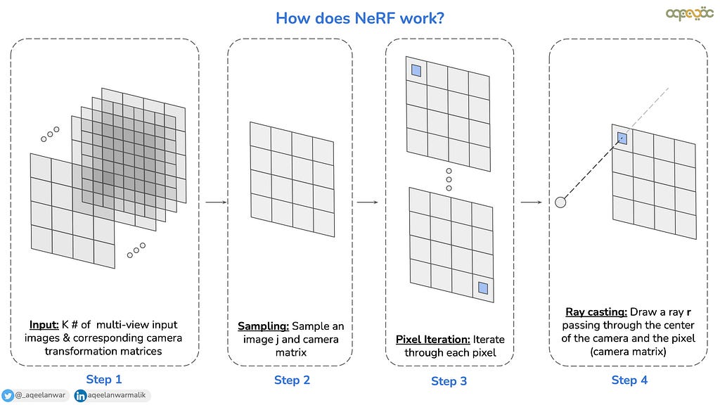
Step 5: Ray Marching
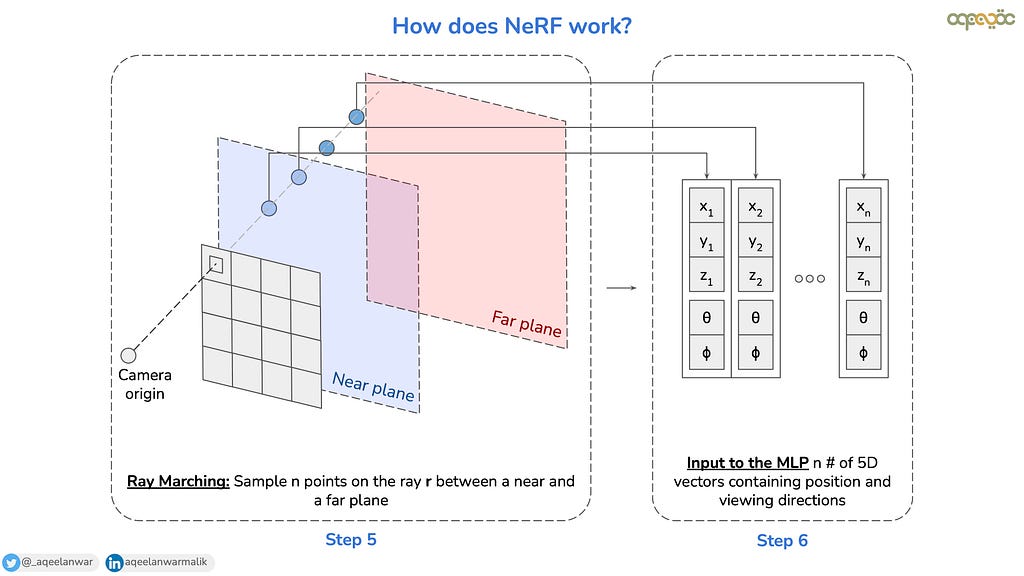
Once the ray is cast, we sample n point along the ray. Theoretically, the ray can extend out infinitely, so to limit the ray we define a near r(t_n) and far plane r(t_f) which are t_n and t_f distance away from the camera center. These planes limit our search space. Only the space within these planes is considered for scene reconstruction, hence the planes need to be defined by the scene under consideration.
Step 6, 7: Multi layer perceptron (MLP)
Now for each pixel in the camera image, we have a viewing direction (θ, φ — which is the same) and n number of 3D points from the scene that lie in that viewing direction ((x1, y1,z1), (x2, y2, z2), …, (xn, yn, zn)). From these parameters, we create n number of 5D vectors which is used as input to the MLP as shown above The MLP then predicts n number of 4D vectors that contain the directional emitted color c (i.e. the RGB color c=(ri, gi, bi) contributed by the 3D position xi, yi, zi towards the pixels when viewed from the direction θi, φi), and a volumetric density σ (a scalar value used to determine the probability of a ray interacting with a particular point in space). σ indicates how “opaque” a point in space is. High values of σ mean that the space is dense (e.g., part of an object), while low values indicate empty or transparent regions.
Formally the MLP F_Θ does the following
where d is the viewing direction (either (θ, φ), or a 3D unit vector) of the ray, and x = (x, y, z) is the 3D position of the sampled point along the ray.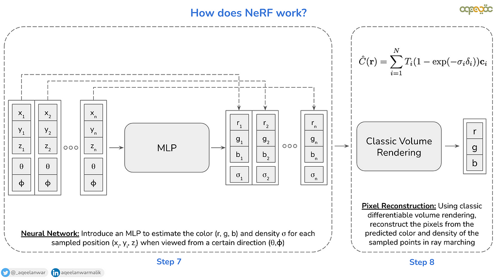
Step 8: Pixel reconstruction
The pixel color is reconstructed by integrating contributions along the ray that passes through the scene. For a ray parameterized as r(t)=o+td, the color C(r) of the ray (and thus the pixel) is computed using the volume rendering equation as follows
where sigma(r(t)) is the volumetric density of the point r(t) on the ray cast, c(r(t), d) is the directional emitted color of the point r(t), t_f and t_n are the limits defined by the near and the far plane. T(t) is the transmittance, representing the probability that light travels from the camera to depth t without being absorbed, and is calculated as follows
Let's first understand what transmittance is. The farther you move along the ray, the higher the probability that the ray is absorbed within the scene. Consequently, the transmittance is determined by the negative exponent of the cumulative volumetric density integrated from the near plane to the point t where the transmittance is being calculated.
Equation 1 can be interpreted as follows: the color of the ray (and hence the pixel) is computed as a weighted sum of the emitted color at each point along the ray. Each point’s contribution is weighted by two factors:
- The probability that the ray reaches the point t without being absorbed (transmittance, T(t))
- The probability that the point contains material capable of emitting or reflecting light (volumetric density, σ(r(t))).
This combination ensures that the rendered color accounts for both the visibility of the point and the physical presence of light-emitting or light-reflecting material.
Since from the MLP, we don't have access to all the points that lie on the ray r(t), we discretized the volume rendering equation above and applied it using the n number of points (determined during the ray marching)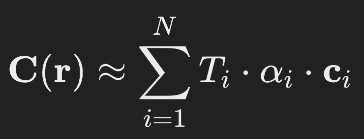
This formula is similar, except that instead of directly using σ as a weight, we use α. While σ represents the volumetric density at a single point in space (which works for continuous spaces), α represents the opacity over a discrete segment of the ray (to take into account the discrete nature of the equation), taking into account both the local density σ and the sampling step size Δti.
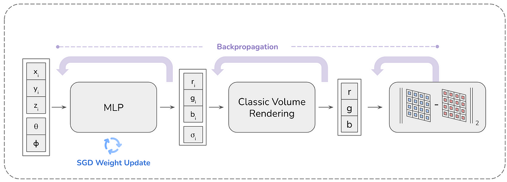
The volume rendering takes the MLP output and calculates the pixel RGB color which is then compared to the input pixel color. An important advantage of the volume rendering equation is its differentiability, enabling the MLP to be efficiently trained through backpropagation.
Steps 9, 10, and 11: Image reconstruction, Loss calculation & Optimization
After estimating the pixel color through volume rendering, the same process is repeated for all pixels in the image to reconstruct the complete image. The reconstructed image is then compared to the input image, and a pixel-wise Mean Squared Error (MSE) loss is computed as follows.
where N is the total number of pixels in the image, C_pred is the predicted pixel color, C_true is the actual pixel color.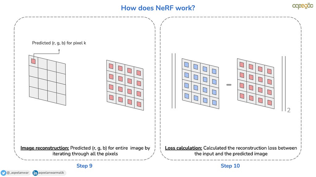
The two primary components involved in reconstructing an image from the input images in NeRF are the MLP and the volume rendering module, both of which are differentiable. This differentiability enables the use of backpropagation to optimize the system. Based on the calculated loss (e.g., pixel-wise Mean Squared Error), the gradient is propagated back through the volume rendering process to the MLP. The weights of the MLP are updated iteratively until the loss converges and the MLP is effectively trained to encode the scene.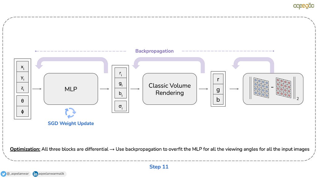
The NeRF paper enhances performance with techniques like stratified sampling, positional encoding, and separate dependencies for volumetric density (σ) and emitted color (c). Stratified sampling ensures robust ray integration, while positional encoding captures high-frequency details by mapping inputs to a higher-dimensional space. σ depends only on spatial position (x), modeling scene geometry, whereas c depends on both position (x) and viewing direction (d), capturing view-dependent effects like reflections. As this is a beginner’s guide, the article will not delve into the details of these techniques, but they can be explored further in the original paper.
Step 12: Rendering image from a novel viewpoint (inference)
Now that we have a trained, scene-specific MLP that overfits to the scene under consideration, we can render 2D images from novel viewpoints. This is achieved by casting rays through each pixel of the target view, sampling points along these rays, and feeding their 3D coordinates and viewing directions into the MLP. The MLP predicts the volumetric density (σ) and emitted color (c) for each sampled point, which are then aggregated using the classical volume rendering equation to compute the final pixel color. By repeating this process for every pixel in the image, the full 2D image is reconstructed, producing a photo-realistic rendering of the scene from the novel view.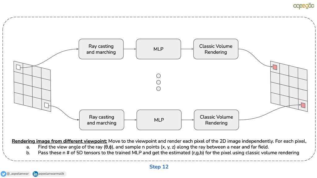
as opposed to other ML approaches of making a generalizable model (foundation models) that can solve a wide range of problems, the MLP in NeRF is trained for specificity. The MLP is overfitted to only work for the given scene (for example an object under consideration)
Summary:
This article provides a visual guide to understanding NeRF for beginners. The article breaks down NeRF’s workflow into 12 simple, easy-to-follow steps. Here’s a summary:
- Input: NeRF requires multi-view images of a scene, along with their corresponding camera matrices.
- Sampling: Start by selecting an image and its camera matrix to begin the process.
- Pixel Iteration: For each pixel in the image, repeat the following steps.
- Ray Casting: Cast a ray r from the camera center through the pixel, as defined by the camera matrix.
- Ray Marching: Sample n points along the ray r, between a near and a far plane.
- Input to the MLP: Construct n 5D vectors, each containing the sampled position (x,y,z) and viewing direction (θ,ϕ), and feed them into the MLP.
- MLP Output: The MLP predicts the color (r, g, b) and volumetric density σ for each sampled point.
- Pixel Reconstruction: Use differentiable volume rendering to combine the predicted color and density of the sampled points to reconstruct the pixel’s color.
- Image Reconstruction: Iterate over all pixels to predict the entire image.
- Loss Calculation: Compute the reconstruction loss between the predicted image and the ground truth input image.
- Optimization: Leverage the differentiable nature of all components to use backpropagation, training the MLP to overfit the scene for all input views.
- Rendering from Novel Viewpoints: Query the trained MLP to generate pixel colors for a new viewpoint and reconstruct the image.
If this article was helpful to you or you want to learn more about Machine Learning and Data Science, follow Aqeel Anwar, or connect with me on LinkedIn. You can also subscribe to my mailing list.
A 12-step visual guide to understanding NeRF (Representing Scenes as Neural Radiance Fields) was originally published in Towards Data Science on Medium, where people are continuing the conversation by highlighting and responding to this story.
What's Your Reaction?




_LuckyStep48_Alamy.jpg?#)


